
Stochastic algorithms in Machine Learning
Published:
This note is an attempt to convey the main ideas and notions of the talk entitled “Stochastic algorithms in Machine Learning” given by Aymeric Dieuleveut (EPFL, Lausanne, Switzerland) during the Stochastic algorithm Day 2017 (Journée algorithmes stochastiques 2017). This conference was held at Université Paris Dauphine (Paris, France) on December 1st, 2017.
Introduction
The goal of supervised Machine Learning algorithms is to predict the values of some unknown variable from known explanatory variables, given a set of observations. Contrary to purely statistical algorithms, no model has to be specified to the algorithm. In many applications, both the number of observations \(n\) and the number of explanatory variables \(d\) can be large. Stochastic algorithms are used in such large scale frameworks to make prediction tractable.
Supervised Machine Learning
Consider an input/output pair \((X,Y)\in\mathcal{X}\times\mathcal{Y}\), \(\mathcal{Y}\subset \mathbb{R}\), with unknown joint distribution \(\rho\). The goal is to find a function \(\theta : \mathcal{X} \rightarrow \mathbb{R}\) such that \(\theta(X)\) is a good prediction for \(Y\). To do so, we consider a loss function \(l : \mathcal{Y}\times \mathbb{R} \rightarrow \mathbb{R}_+\) such that \(l(y,\theta(x))\) is the loss from predicting \(y\) using \(\theta(x)\).
The Generalization risk (or true risk) is defined as
\[\begin{aligned} \mathcal{R}(\theta):=\mathbb{E}_\rho[l(Y, \theta(X))] \end{aligned}\]and is a measure of the quality of \(\theta(X)\) as a predictor of \(Y\). Given that \(\rho\) is unknown, we can’t in general compute directly this risk.
Starting from a set of \(n\) observations \((x_i,y_i)\in\mathcal{X}\times \mathcal{Y}\), \(i\in[\![1,n]\!]\) assumed to be i.i.d. with (unknown) distribution \(\rho\), the Empirical risk (or training error) is defined as
\[\begin{aligned} \widehat{\mathcal{R}}(\theta)=\frac{1}{n}\sum\limits_{i=1}^nl(y_i,\theta(x_i)) \end{aligned}\]and is used in practice to choose the best predictor \(\theta\), considering the observations and some regularisation factor \(\Omega(\theta)\), through the Empirical Risk Minimisation (ERM) problem :
\[\begin{aligned} \theta^* = \min\limits_\theta \left[\widehat{\mathcal{R}}(\theta) + \mu\Omega(\theta)\right]=\min\limits_\theta \left[\frac{1}{n}\sum\limits_{i=1}^nl(y_i,\theta(x_i)) + \mu\Omega(\theta)\right] \end{aligned}\]From now on, linear functions are considered. We reparametrize :
\[\begin{aligned} \theta(X) = \langle \theta, \Phi(X) \rangle, \quad \theta\in\mathbb{R}^d,\quad \Phi : \mathcal{X}\rightarrow \mathbb{R}^d \end{aligned}\]The high number of explanatory variables \(d\) pushes us to choose first order algorithm for the ERM, namely the Gradient Descent algorithm. For instance, choosing second order algorithms such as the Newton-Raphson algorithm, would imply to compute a \(d\times d\) matrix at each iteration: the Hessian of the overall loss.
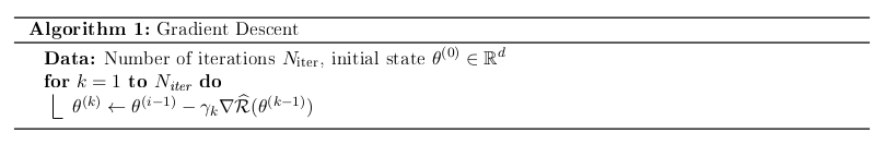
Each iteration implies \(\mathcal{O}(dn)\) operations for the computation of the Gradient. Stochastic algorithms are used to reduce this number. In particular, the Stochastic Gradient algorithm only implies \(\mathcal{O}(d)\) operations per iteration.
Stochastic Gradient descent
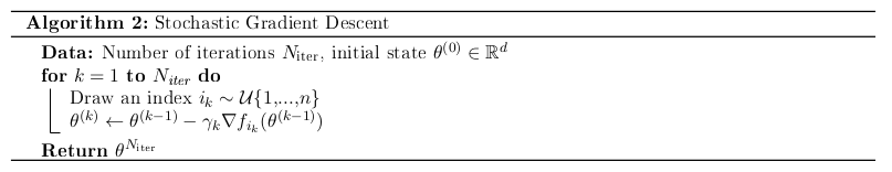
The idea of Stochastic Gradient Descent (SGD) is to replace, at each iteration \(k\), the gradient of the empirical risk \(\nabla\widehat{\mathcal{R}}(\theta^{(k-1)})\) by a gradient function \(g^{(k)}(\theta^{(k-1)})\) cheaper to compute and verifying :
\[\begin{equation} \mathbb{E}[g^{(k)}(\theta^{(k-1)})\vert \mathcal{F}_{k-1} ]=\nabla\widehat{\mathcal{R}}(\theta^{(k-1)}) \tag{1}\label{SGD_origin} \end{equation}\]for a filtration \((\mathcal{F}_{k})_{k\ge 0}\) such that \(\theta^{(k)}\) is \(\mathcal{F}_k\)-measurable.
Notice that the empirical risk can be written :
\[\begin{aligned} \widehat{\mathcal{R}}(\theta)=\frac{1}{n}\sum\limits_{i=1}^nf_i(\theta), \quad f_i : \theta \mapsto l(y_i,\theta(x_i)) \end{aligned}\]Consider the filtration \(\mathcal{F}_k=\sigma\left((x_i,y_i)_{1\le i \le n}, (i_j)_{0\le j \le k}\right)\) where \((i_j)_{j \ge 0}\) are independent indices uniformly sampled from \([\![1,n]\!]\). It can be shown that \(g^{(k)}:=\nabla{f_{i_k}}\) verifies \eqref{SGD_origin}. The SGD algorithm is then described below.
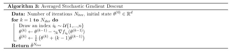
To reduce noise effect due to the proxy used for the gradient computation step, we may take the average of all states \(\theta^{(k)}\) as an estimator of the optimum, instead of just last one. This average \(\bar\theta^{(k)}\) may be computed "on line", meaning that it can be updated at each iteration without requiring the storage of all previous states.
Assume the following properties for the loss function \(l\) :
\(l\) is \(L\)-smooth, i.e. \(L\) is a lower bound of the eigenvalues of the Hessian matrix of \(l\) at any point
\(l\) is \(\mu\)-strongly convex, i.e. \(\mu\) is a upper bound of the eigenvalues of the Hessian matrix of \(l\) at any point
In particular, at any points of evaluation \((u,v)\), \(l\) verifies :
\[\begin{aligned} \langle \nabla l(v), u-v\rangle + \mu\Vert u-v\Vert^2 \le l(u)-l(v) \le \langle \nabla l(v), u-v\rangle + L\Vert u-v\Vert^2 \end{aligned}\]With some additional assumptions on the observations \(\Phi(x_i)\) (bounded variance and invertible experimental covariance matrix), it can be shown that then empirical risk also verifies those two properties.\
Importance of the learning rate \(\gamma_k\)
For smooth and convex problems, it was shown that almost surely, \(\theta_k \rightarrow \theta^*\) if
\[\begin{aligned} \sum\limits_{k=1}^\infty \gamma_k =\infty \quad \sum\limits_{k=1}^\infty \gamma_k^2 =\infty \end{aligned}\]and asymptotically, for \(\gamma_k =\frac{\gamma_0}{k}, \gamma_0 \ge \frac{1}{\mu}\), \(\sqrt{k}(\theta_k - \theta^*) \mathop{\rightarrow}\limits^d \mathcal{N}(0,V)\).
Comparison of convergence rate
The convergence rate of an optimization algorithm measures the speed of convergence of torwards the solution of the problem. It is, with our notations, given by the speed at which \((\widehat{\mathcal{R}}(\theta^{(k)}))_{k\ge 0}\) converges to the minimum of \(\widehat{\mathcal{R}}\). Let’s compare the convergence rate of GD and (A)SGD for both convex and strongly convex functions.
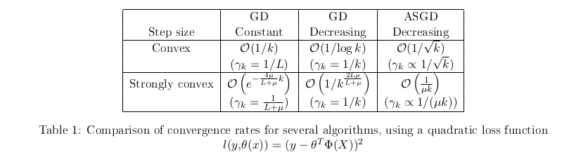
One one hand, GD can converge much master to the optimum \(\theta^*\) than SGD. But on the other hand, each iteration of GD is more costly (by a factor \(n\)) than an iteration of SGD. The idea is to come up with a way to get the best of both worlds.
Stochastic Average Gradient
The Stochastic Average Gradient algorithm, is a SGD algorithm in which the at each iteration, the full gradient \(g^{(k)}\) given by
\[\begin{aligned} g^{(k)}=\frac{1}{n}\sum\limits_{i=1}^n\nabla f_i(\theta^{(k_i)}), \quad k_i\in[\![0,k]\!] \end{aligned}\]is updated through \(i_k\)-th term of the sum, where \(i_k\) is once again an index randomly chosen at each iteration. The term \(\nabla f_{i_k}(\theta^{(k_{i_k})})\) is replaced by \(\nabla f_{i_k}(\theta^{(k)})\) in the sum, where \((\theta^{(k)})_{k\ge 0}\) are obtained through a GD iteration step in which the gradient is replaced by \(g^{(k)}\).
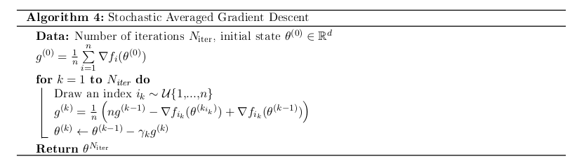
This algorithm has the same update cost as SGD but the averaged gradient \(g^{(k)}\) has a smaller variance than the gradient used in SGD. Moreover, choosing a constant step size \(\gamma_k=\frac{1}{2nL}\) yields a convergence rate of \(\mathcal{O}((1- \frac{1}{8Ln})^k)\). However, it is required to store at all time \(n\) elementary gradients \(\nabla f_i(\theta^{(k_i)})\) as one of them is systematically used in the updating step of \(g^{(k)}\).
Generalization risk
Using the Empirical risk to determine the best predictor \(\theta^*\) given the data arises several problems. First, to avoid over-fitting, a regularisation function must be set. Then, the number of iterations needed to achieve the optimum is hard to predict.
On the other hand, using Generalisation risk yields a more general approach given that it measures how accurately we may predict outcome values for previously unseen data (through the expectation). Therefore, regularisation is no longer needed. As we may see now, SGD can be used to minimise the generalisation risk, even though its expression is unknown.
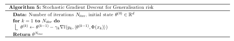
SGD would replace computations of the gradient of the Generalisation risk \(\nabla\mathcal{R}(\theta^{(k-1)})\) by a proxy \(g^{(k)}(\theta^{(k-1)})\) verifying :
\[\begin{equation} \mathbb{E}[g^{(k)}(\theta^{(k-1)})\vert \mathcal{F}_{k-1} ]=\nabla{\mathcal{R}}(\theta^{(k-1)})=\mathbb{E}_\rho[\nabla l(Y, \langle\theta^{(k-1)}, \Phi(X)\rangle)] \tag{2}\label{SGD_origin_GR} \end{equation}\]Considering that the examples \((x_i,y_i)_{1\le i \le n}\) are i.i.d from \(\rho\), we can take for \(g^{(k)}\) at iteration \(1\le k \le n\):
\[\begin{aligned} g^{(k)}(\theta^{(k-1)})=\nabla l(y_k, \langle\theta^{(k-1)}, \Phi(x_k)\rangle) \end{aligned}\]and the filtrations \(\mathcal{F}_{k-1}=\sigma((x_i,y_i)_{1\le i \le k})\). Therefore there is a single pass through the data in this algorithm, and exactly \(n\) iterations are needed. Hence, with a convex (resp. strongly convex) loss function and a constant step size, it has a convergence rate of \(\mathcal{O}(1/\sqrt{n})\) (resp. \(\mathcal{O}(1/(\mu n))\)).
Beyond Least squares for Generalisation risk : SGD as a Markov chain
All the convergence rates previously mentioned are related to the use of a quadratic loss function \((x,y) \mapsto l(x,\theta(x))=(y-\theta^T\Phi(x))^2\). When using other loss functions, the results don’t hold, and the SGD may even not converge! For instance, for the logistic loss \((x,y) \mapsto l(x,\theta(x))=\log\left(1+\exp(y-\theta^T\Phi(x))\right)\) averaged SGD with constant step size \(\gamma\) happened to yield convergence rates of \(\mathbb{E}[\bar\theta^{(k)}-\theta^*]=\mathcal{O}(\gamma)\) (therefore independent of the number of iterations...).
To understand this problem and come up with solutions, SGD (with constant step size) was formulated as an homogeneous Markov chain.
Consider a \(L\)-smooth and \(\mu\)-strongly convex risk \(\mathcal{R}\). Then SGD with a step size \(\gamma\) may be seen as the generation of a sequence \((\theta^{(k)}_\gamma)_{k\ge 0}\) with recurrence :
\[\begin{aligned} \theta^{(k)}_\gamma=\theta^{(k-1)}_\gamma-\gamma\underbrace{\left(\nabla\mathcal{R}(\theta^{(k-1)}_\gamma)+\varepsilon^{(k)}(\theta^{(k-1)}_\gamma) \right)}_{=g^{(k)}(\theta^{(k-1)}_\gamma)} \end{aligned}\]where \((\varepsilon^{(k)})_{k\ge 0}\) are i.i.d. random noises verifying for any \(\theta\), \(\mathbb{E}[\varepsilon^{(k)}(\theta)\vert \mathcal{F}_{k-1}]=0\) for the same filtrations as in \eqref{SGD_origin_GR}. Introduced like this, \((\theta^{(k)}_\gamma)_{k\ge 0}\) is a homogeneous Markov chain, which allow us to understand the general behaviour of the SGD.
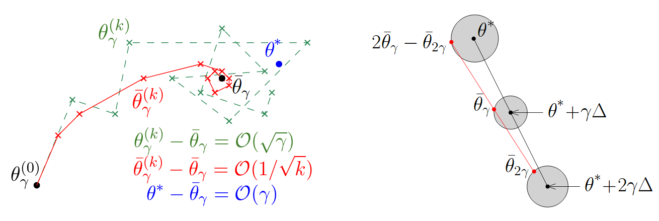
Indeed, this Markov chain will converge exponentially fast to its (unique) stationary distribution \(\pi_\gamma\). Consequently, this sequence (and therefore the SGD) does not converge to a point, but rather will (asymptotically) oscillate around the mean \(\bar\theta_\gamma = \mathbb{E}_{\pi_\gamma}[\theta]\) with an average magnitude \(\gamma^{1/2}\). On the other hand, considering as an output the average \(\bar\theta^{(k)}_\gamma\) of the \(k+1\) states \(\lbrace\theta^{(i)} :0\le i \le k \rbrace\), we can prove (central limit theorem) that with rate \(\mathcal{O}(1/\sqrt{k})\) :
\[\begin{aligned} \bar\theta^{(k)}_\gamma \mathop{\rightarrow}\limits_{k\rightarrow \infty}^{L^2} \bar\theta_\gamma = \mathbb{E}_{\pi_\gamma}[\theta] \end{aligned}\]Therefore the output of the averaged SGD is known to converge at a given rate to \(\bar\theta_\gamma\), which may different than the optimum \(\theta^*\). The error between the output of the SGD \(\theta^{(k)}_\gamma\) and the optimum can be decomposed:
\[\begin{aligned}\theta^{(k)}_\gamma-\theta^*=\underbrace{\theta^{(k)}_\gamma-\bar\theta_\gamma}_{\mathcal{O}(1/\sqrt{k})}+\underbrace{\bar\theta_\gamma - \theta^*}_{\text{independent of k}} \end{aligned}\]Notice that if we take \(\theta^{(0)}_\gamma \sim \pi_\gamma\), then by definition of \(\pi_\gamma\),
\[\begin{aligned} \theta^{(0)}_\gamma -\gamma\left(\nabla\mathcal{R}(\theta^{(0)}_\gamma)+\varepsilon^{(1)}(\theta^{(0)}_\gamma) \right)=\theta^{(1)}_\gamma \sim \pi_\gamma \end{aligned}\]Hence, by taking the expectation under \(\pi_\gamma\) we get :
\[\begin{aligned} \mathbb{E}_{\pi_\gamma}[\nabla\mathcal{R}(\theta^{(0)}_\gamma)]=0 \end{aligned}\]and recalling the expression of \(\mathcal{R}\) we get
\[\begin{aligned} \mathbb{E}_{\pi_\gamma}[\nabla\mathcal{R}(\theta)]=\mathbb{E}_{\pi_\gamma}\left[\mathbb{E}_\rho[\nabla l(Y, \Phi(X)^T\theta)]\right]=\mathbb{E}_\rho\left[\mathbb{E}_{\pi_\gamma}[\nabla l(Y, \Phi(X)^T\theta)]\right]=0 \end{aligned}\]In particular, in the quadratic loss case, given that \(\theta \mapsto \nabla l(Y, \Phi(X)^T\theta)=2(Y-\Phi(X)^T\theta)\Phi(X)\) is a linear function of \(\theta\), we have
\[\begin{aligned} \mathbb{E}_\rho\left[\mathbb{E}_{\pi_\gamma}[\nabla l(Y, \Phi(X)^T\theta)]\right]=\mathbb{E}_\rho\left[\nabla l(Y, \Phi(X)^T\mathbb{E}_{\pi_\gamma}[\theta])\right]=\nabla\mathcal{R}(\mathbb{E}_{\pi_\gamma}[\theta])=0 \end{aligned}\]And therefore,
\[\begin{aligned} \bar\theta_\gamma = \mathbb{E}_{\pi_\gamma}[\theta]=\theta^*. \end{aligned}\]We retrieve the fact that in the quadratic loss case, the averaged SGD converges to the optimum at rate \(\mathcal{O}(1/\sqrt{k})\).
However, in the general case, using a Taylor expansion of \(\mathcal{R}\), we can only show that
\[\begin{equation} \bar\theta_\gamma = \theta^*+\gamma C +\mathcal{O}(\gamma^2) \tag{3}\label{gen_output} \end{equation}\]where \(C\) is a constant independent of \(\gamma\). Therefore the averaged SGD will only converge to a point "near" the optimum. To get a better estimate of \(\theta^*\), we can use Richardson extrapolation. For instance, for two terms, the idea is to run SGD with rates \(\gamma\) and \(2\gamma\), which will yield estimates of \(\bar\theta_\gamma\) and \(\bar\theta_{2\gamma}\). Then, from \eqref{gen_output}, notice that :
\[\begin{aligned} 2\bar\theta_\gamma - \bar\theta_{2\gamma} = \theta^* + \mathcal{O}(\gamma^2) \end{aligned}\]is a better estimate of \(\theta^*\). This approach can simply be generalized to more terms (runs of the SGD).
References
Bach, F. (2012). Stochastic gradient methods for machine learning. Technical report. INRIA-ENS, Paris, France. Available at http://www.di.ens.fr/~fbach/fbach_sgd_online.pdf
Dieuleveut, A., Durmus, A., Bach, F. (2017). Bridging the Gap between Constant Step Size Stochastic Gradient Descent and Markov Chains. arXiv preprint arXiv:1707.06386.
Dieuleveut, A. (2017, December). Stochastic algorithms in Machine Learning. Paper presented at "Journée algorithmes stochastiques", Université Paris Dauphine, Paris, France.
Roux, N. L., Schmidt, M., Bach, F. R. (2012). A stochastic gradient method with an exponential convergence rate for finite training sets. In Advances in Neural Information Processing Systems (pp. 2663-2671).